The goal of the tba package is to provide easy access to match data for events run in the first robotics division. Access is based on the Read API v3 of The Blue Alliance.
Installation
You can install the development version of tba from GitHub with:
# install.packages("pak")
pak::pak("heike/tba")
In order to access the API of The Blue Alliance, you will need to sign up for a (free) account. Then run
tba::set_api_key(key = "jnn1ZiUfqPuA9UJyV9EVa3jtL5qudBBlYXKPEVQDeQgQgz5L8BypwjTzVKxtCs3W")
# key is not valid, get your own!
Example
This is a basic example which shows you how to solve a common problem:
library(tba)
## basic example code

# Team Neutrino has team code `frc3928`
get_records("team/frc3928")
#> # A tibble: 1 × 11
#>   city  country key     name        nickname postal_code rookie_year school_name
#>   <chr> <chr>   <chr>   <chr>       <chr>    <chr>             <int> <chr>
#> 1 Ames  USA     frc3928 Iowa 4-H F… Team Ne… 50011              2012 4-H
#> # ℹ 3 more variables: state_prov <chr>, team_number <int>, website <chr>

# In the 2024 season, the team attended the following events:
events <- get_records("team/frc3928/events/2024")
events$name
#> [1] "Cow Town Throwdown"        "Galileo Division"
#> [3] "Iowa Regional"             "Clash in the Corn"
#> [5] "Central Missouri Regional"
events$event_code
#> [1] "cttd"  "gal"   "iacf"  "iawes" "mose"
Access Score Data from a Competition
The matches from Clash in the Corn can be accessed using the event code 2024iawes:
library(dplyr)
matches <- get_records("event/2024iawes/matches")
count(matches, comp_level)
#> # A tibble: 3 × 2
#>   comp_level     n
#>   <chr>      <int>
#> 1 f              2
#> 2 qm            22
#> 3 sf             5
# 22 qualifying matches
# 5 semi-finals
# 2 finals
The function get_match_details turns the records into a more manageable form by turning the match-based rows from the get_records results into team-based results, i.e. every row corresponds to the detailed scores of each team in each one of the matches:
scores <- get_match_details(matches)
head(scores %>% select(comp_level, match_number, set_number, alliance, team_key, score, ends_with("Points")))
#> # A tibble: 6 × 25
#>   comp_level match_number set_number alliance team_key score adjustPoints
#>   <chr>             <int>      <int> <chr>    <chr>    <int>        <int>
#> 1 f                     1          1 blue     frc9998     38            0
#> 2 f                     1          1 blue     frc6419     38            0
#> 3 f                     1          1 blue     frc4646     38            0
#> 4 f                     2          1 blue     frc9998     44            0
#> 5 f                     2          1 blue     frc6419     44            0
#> 6 f                     2          1 blue     frc4646     44            0
#> # ℹ 18 more variables: autoAmpNotePoints <int>, autoLeavePoints <int>,
#> #   autoPoints <int>, autoSpeakerNotePoints <int>, autoTotalNotePoints <int>,
#> #   endGameHarmonyPoints <int>, endGameNoteInTrapPoints <int>,
#> #   endGameOnStagePoints <int>, endGameParkPoints <int>,
#> #   endGameSpotLightBonusPoints <int>, endGameTotalStagePoints <int>,
#> #   foulPoints <int>, teleopAmpNotePoints <int>, teleopPoints <int>,
#> #   teleopSpeakerNoteAmplifiedPoints <int>, teleopSpeakerNotePoints <int>, …
Calculate a team’s contribution to an outcome
The function get_ranking_by allows a ranking of each team (not the alliance!) by any numeric variable. It only makes sense to use matches from the qualifying round. The resulting number is an estimate of the team’s contribution to the chosen measurement. When using get_ranking_by with the score from the qualifying matches, the resulting coefficients for the ranking is the Offesnive Power Rating (OPR) - as published on the TBA API under insights.
# ranking by OPR
scores %>% filter(comp_level=="qm") %>%
  get_ranking_by(score)
#> # A tibble: 12 × 3
#>    team_key     n `rating(score)`
#>    <chr>    <int>           <dbl>
#>  1 frc3928     11           24.8
#>  2 frc5041     11           23.8
#>  3 frc4646     11           17.2
#>  4 frc525      11           16.5
#>  5 frc6419     11           15.4
#>  6 frc6317     11           14.3
#>  7 frc9999     11           13.7
#>  8 frc9997     11            9.06
#>  9 frc9998     11            7.14
#> 10 frc9996     11            2.86
#> 11 frc967      11            2.58
#> 12 frc9995     11            2.32
It makes sense, to not include points from fouls (assuming that it is hard to make another team foul one’s alliance):
no_fouls <- scores %>% filter(comp_level == "qm") %>%
  get_ranking_by(score - foulPoints)
head(no_fouls)
#> # A tibble: 6 × 3
#>   team_key     n `rating(score - foulPoints)`
#>   <chr>    <int>                        <dbl>
#> 1 frc3928     11                         23.6
#> 2 frc4646     11                         19.4
#> 3 frc5041     11                         19.1
#> 4 frc525      11                         17.5
#> 5 frc6317     11                         12.7
#> 6 frc6419     11                         11.9
Most of the time, the resulting ranking should be quite similar, but differences in these rankings might give some insight as to whether some teams profitted from being fouled during the qualification round. In this example, most of the rankings stay the same, but the 2nd and the 3rd team switch places: frc5041 seems to have benefitted during the qualifying matches more from their opponents’ fouls than frc4646. Their rating of contribution to the team’s score without counting fouls is quite similar.
scores %>% filter(comp_level=="qm") %>%
  get_ranking_by(score-foulPoints)
#> # A tibble: 12 × 3
#>    team_key     n `rating(score - foulPoints)`
#>    <chr>    <int>                        <dbl>
#>  1 frc3928     11                       23.6
#>  2 frc4646     11                       19.4
#>  3 frc5041     11                       19.1
#>  4 frc525      11                       17.5
#>  5 frc6317     11                       12.7
#>  6 frc6419     11                       11.9
#>  7 frc9999     11                       10.7
#>  8 frc9997     11                        6.37
#>  9 frc9998     11                        5.96
#> 10 frc967      11                        2.44
#> 11 frc9996     11                       -0.409
#> 12 frc9995     11                       -2.54
Comparing Multiple Outcomes
By comparing the two measures visually we also see, that the big gap between the top two teams and the other teams suggested by the OPR ranking, turns into a group of four teams with a gap to the remaining teams:
library(tidyverse)
library(ggplot2)

# combine the OPR with the ranking not including fouls:
all_points <- scores %>% get_ranking_by(score, score-foulPoints)
all_points %>% ggplot(aes(x = `rating(score)`, y = `rating(score - foulPoints)`)) +
  geom_point() + xlab("OPR") +
  ggrepel::geom_label_repel(aes(label = team_key), size=3, alpha = 0.6) +
  geom_rug(length = unit(0.03, "npc")) +
  scale_y_continuous(expand = c(0.2, 0.2)) +
  scale_x_continuous(expand = c(0.2, 0.2)) +
  coord_equal()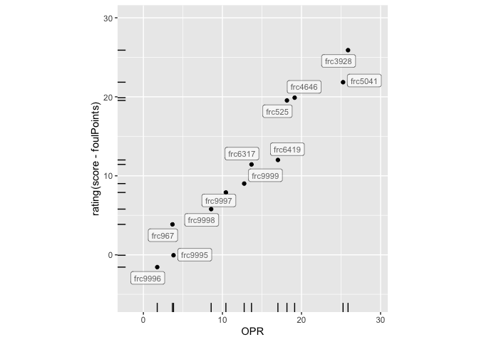
Scatterplot of team contributions measured in OPR (x axis) and to the score without foul points (y axis).
Worst fouling team
Any of the details going into the score can be used as outcome measurement. The number of points given to the opponent because of a team’s foul is determined (in the 2024 season) as 5 points for a foul and 2 points for a technical foul. The list below is sorted from worst offenders to least offenders. A negative number might be interpreted as a team’s ability to provoke fouls from the opponents.
scores %>% filter(comp_level=="qm") %>%
  get_ranking_by(2*foulCount+5*techFoulCount)
#> # A tibble: 12 × 3
#>    team_key     n `rating(2 * foulCount + 5 * techFoulCount)`
#>    <chr>    <int>                                       <dbl>
#>  1 frc9998     11                                      6.06
#>  2 frc9997     11                                      4.91
#>  3 frc6317     11                                      2.60
#>  4 frc525      11                                      2.38
#>  5 frc967      11                                      2.25
#>  6 frc9995     11                                      2.22
#>  7 frc3928     11                                      1.86
#>  8 frc9999     11                                      1.18
#>  9 frc4646     11                                      0.917
#> 10 frc9996     11                                      0.146
#> 11 frc6419     11                                      0.0238
#> 12 frc5041     11                                     -1.62
Best at categories
detailed <- scores %>% filter(comp_level=="qm") %>%
  get_ranking_by(score, score - foulPoints, autoPoints, teleopPoints, -1*(2*foulCount+5*techFoulCount))

# add the tba rating to the mix:
tba_rating <- tba_ranking("2024iawes")
detailed <- detailed %>% left_join(tba_rating %>% select(team_key, TBA=rank), by="team_key")
Taking more measures into account, we can see in the parallel coordinate plot below, that the third place TBA ranking for team frc9999 is not backed up by a similar high performance in the contribution to the score, which is indicative of a lot of luck and/or strategy in the qualifying matches. On the other hand, team frc4646 is in the top three performing teams except for their TBA ranking, indicating that they would be a great pick for any alliance. Similarly, team frc525 would make a good contributing partner in an alliance.
library(ggpcp)


 detailed %>%
   mutate(
     TBA = max(TBA)-TBA,
    team_key = reorder(factor(team_key), TBA)
    ) %>%
   pcp_select(team_key, TBA, starts_with("rating"), team_key) %>%
   pcp_scale() %>%
   ggplot(aes_pcp()) +
   geom_pcp() +
   geom_pcp_labels(size=3) +
   xlab("") + ylab("") +
   theme(axis.text.x = element_text(angle=30, hjust=1))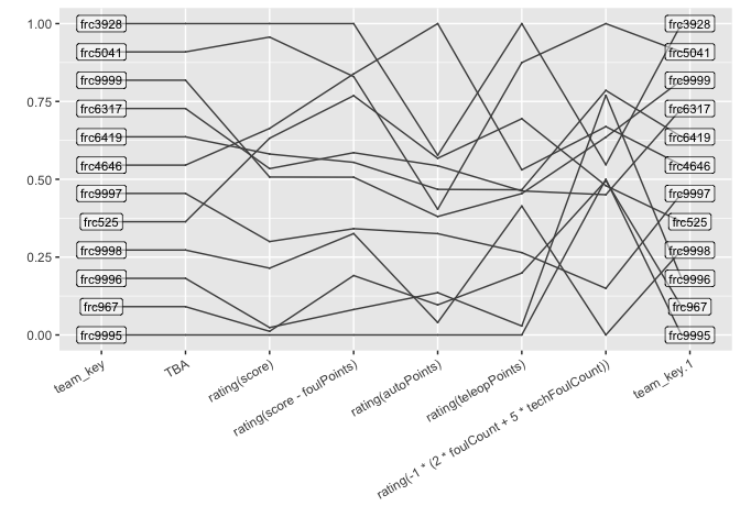
Parallel Coordinate Plot of multiple measures showing different aspects of a team’s contribution. Higher is better for all measures.