handbook

The goal of the package handbook is to provide data for some infrastructure to create graphics.

Installation

You can install the development version of handbook like so:

remotes::install_github("heike/handbook")

Example

This is a basic example which shows you how to solve a common problem:

# Setting up all packages for the examples
library(handbook)
#> Loading required package: ggplot2
library(tidyverse)
#> ── Attaching packages ─────────────────────────────────────── tidyverse 1.3.1 ──
#> ✔ tibble  3.1.7     ✔ dplyr   1.0.9
#> ✔ tidyr   1.2.0     ✔ stringr 1.4.0
#> ✔ readr   2.1.2     ✔ forcats 0.5.1
#> ✔ purrr   0.3.4
#> ── Conflicts ────────────────────────────────────────── tidyverse_conflicts() ──
#> ✖ dplyr::filter() masks stats::filter()
#> ✖ dplyr::lag()    masks stats::lag()
library(patchwork)
library(glue)

## basic example code

Color schemes

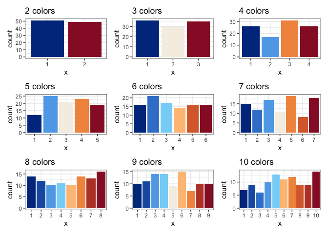
Six sequential color schemes (palette = 1:6, type = "seq") and three divergent color schemes (palette = 1:3, type = "div") were implemented based on IES colors:

scale_fill_nces
#> function (..., type = "seq", palette = 1, direction = -1, aesthetics = "fill") 
#> {
#>     ggplot2::discrete_scale(aesthetics, "nces", nces_pal(type, 
#>         palette, direction), ...)
#> }
#> <bytecode: 0x7fb367df6350>
#> <environment: namespace:handbook>
scale_colour_nces
#> function (..., type = "seq", palette = 1, direction = 1, aesthetics = "colour") 
#> {
#>     ggplot2::discrete_scale(aesthetics, "nces", nces_pal(type, 
#>         palette, direction), ...)
#> }
#> <bytecode: 0x7fb366b024c0>
#> <environment: namespace:handbook>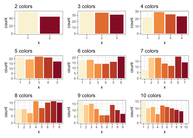

Sequential Color Scheme

#> Warning in choose_n(colors, n, type): chosen color palette only has 9 colors.

Divergent Color Scheme

Maps

The statesmaps object consists of polygons and hex shapes describing each state. Additionally, state names, abbreviations and fips codes are provided for linkage with data sources.

head(statesmaps)
#> # A tibble: 6 × 8
#>   state_name state_abbv state_fips piece hole  group     polygon  hexagon 
#>   <chr>      <chr>      <chr>      <dbl> <lgl> <fct>     <list>   <list>  
#> 1 Alabama    AL         01             1 FALSE Alabama.1 <tibble> <tibble>
#> 2 Alabama    AL         01             2 FALSE Alabama.2 <tibble> <tibble>
#> 3 Alabama    AL         01             3 FALSE Alabama.3 <tibble> <tibble>
#> 4 Alabama    AL         01             4 FALSE Alabama.4 <tibble> <tibble>
#> 5 Alaska     AK         02             1 FALSE Alaska.1  <tibble> <tibble>
#> 6 Alaska     AK         02             2 FALSE Alaska.2  <tibble> <tibble>

As an example to acquire data from the US Census Bureau we can use the code below, thanks to Kyle Walker’s amazing tidycensus package:

library(tidyverse)
library(tidycensus)
census_key <- "place your API key here"
#census_api_key(census_key)

# H012001 encodes the average houshold size
hh10 <- get_decennial(geography = "state",
                       variables = "H012001",
                       year = 2010)
#> Getting data from the 2010 decennial Census
#> Using Census Summary File 1
map_values <- statesmaps %>% left_join(hh10, by = c("state_name" = "NAME"))

Once the data is joined with the mapping information, we can draw choropleth maps or hexbin maps:

map_values %>% unnest(col=polygon) %>%
  ggplot(aes( x = long, y = lat, group = group, fill=value)) +
  geom_polygon(colour = "grey50", size=0.1) +
  #  geom_text (aes(label=id)) +
  theme_void () +
  coord_map () +
  scale_fill_gradient2("Avg. Houshold size", midpoint=median(hh10$value))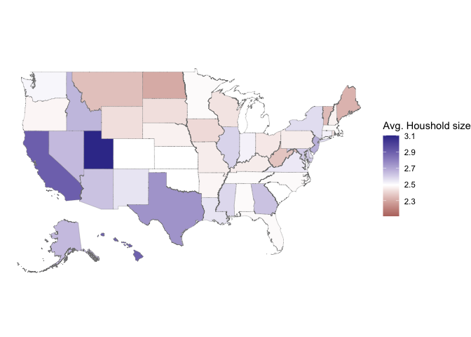

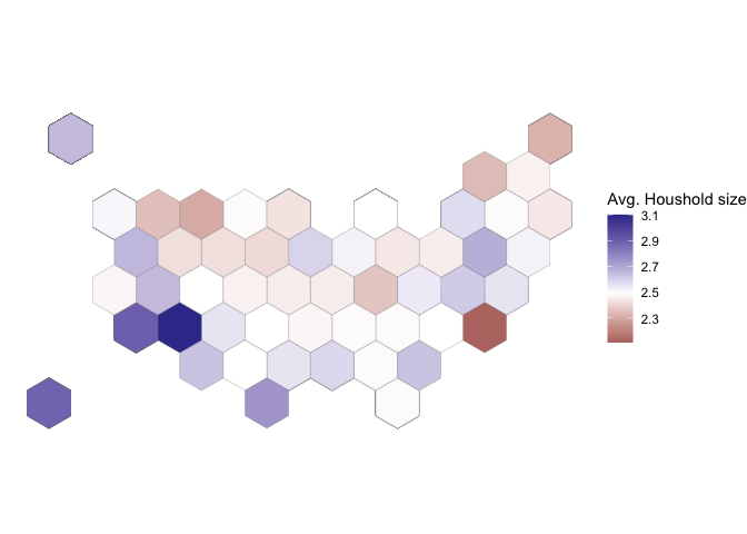
Note that only in the hexbin diagram we get to see the nation’s territory with the smallest average household size: DC residents report in the 2010 census an average household size of 2.1 persons.

map_values %>% unnest(col=hexagon) %>%
  ggplot(aes( x = long, y = lat, group = group, fill=value)) +
  geom_polygon(colour = "grey50", size=0.1) + 
  theme_void () +
  coord_map () +
  scale_fill_gradient2("Avg. Houshold size", midpoint=median(hh10$value))