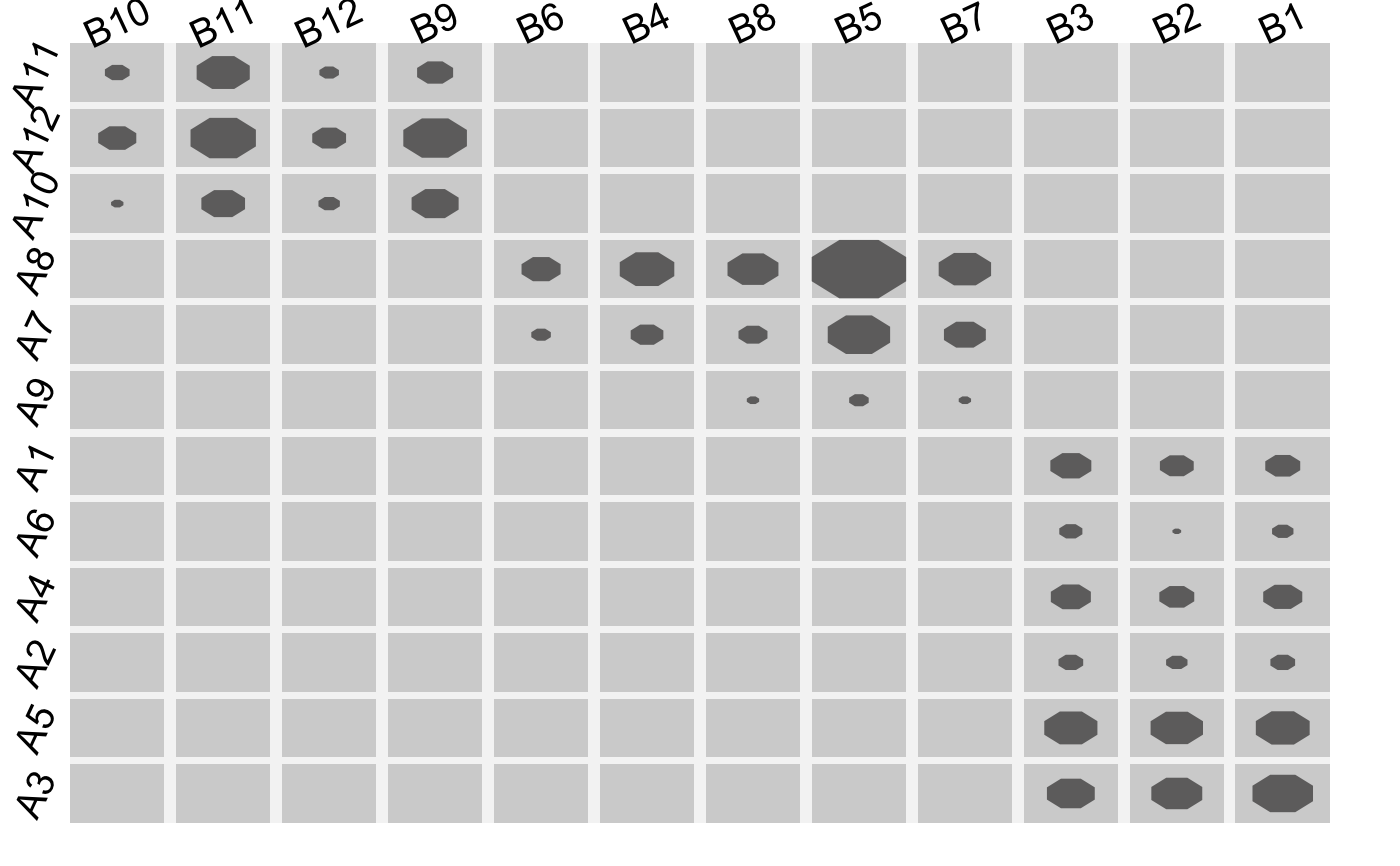
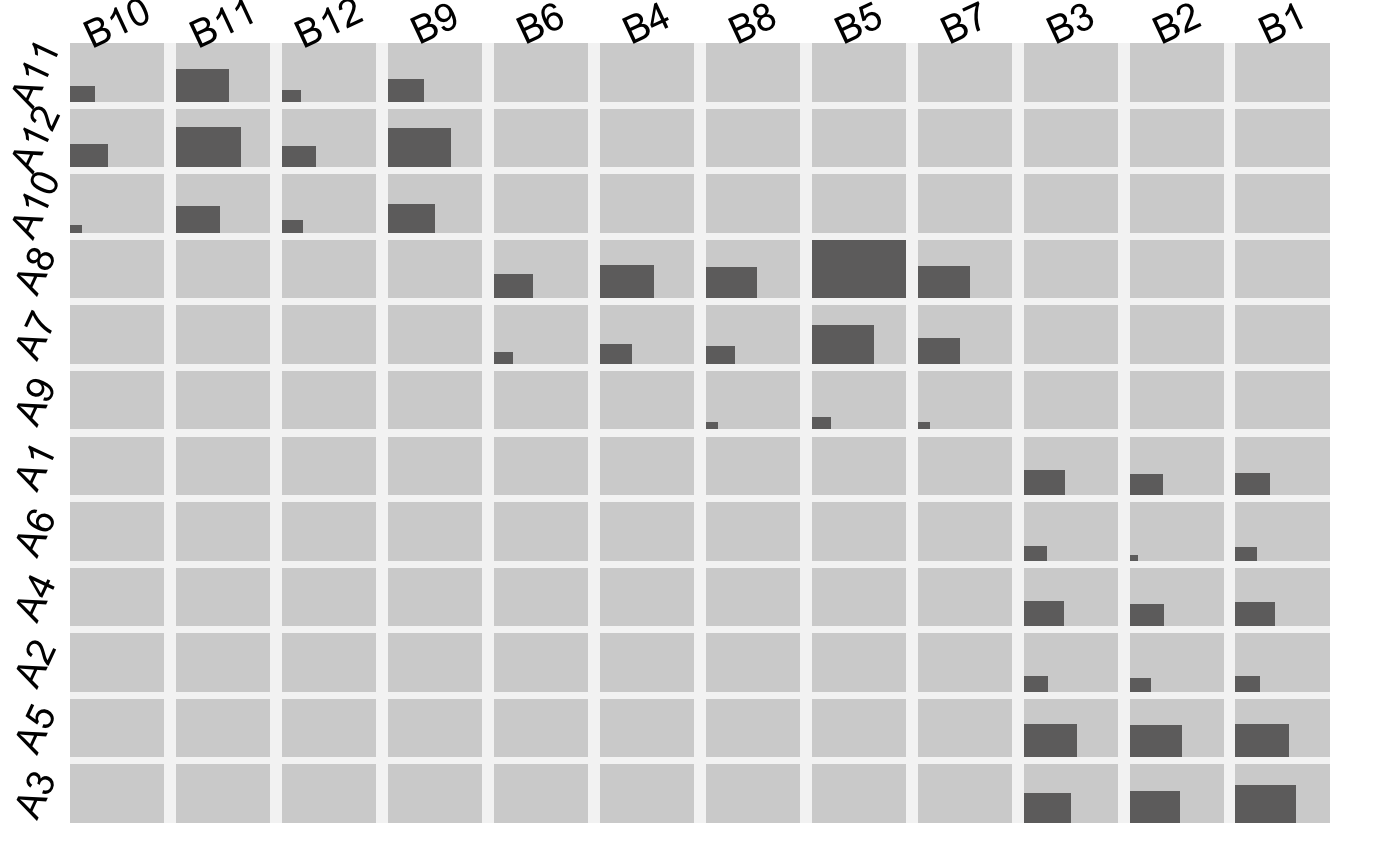
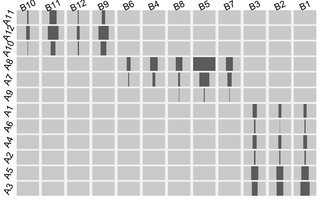
fluctuation diagrams

Create a fluctuation diagram from a multidimensional table.

fluctile(tab, dir = "b", just = "c", hsplit = FALSE, shape ="r", gap.prop = 0.1,
   border = NULL, label = TRUE, lab.opt = list(), add = FALSE, maxv = NULL,
   tile.col = hsv(0.1,0.1,0.1,alpha=0.6), bg.col = ifelse(add,NA,"lightgrey"),
   tile.border = NA, vp = NULL, ...  )

Arguments

tab	The table which is to be plotted.
dir	The bar/rectangle direction: "v" and "h" stand for vertical or horizontal bars. "b" stands for "both" and leads to standard fluctuation diagrams with quadratic rectangles. Use "n" for a same-binsize-plot
just	A shortcut version of the argument used in grid for the anchorpoint of the rectangles: "rb" is equivalent to c("right", "bottom"), "t" is equivalent to "ct" or c("centre", "top") and so on. See examles.
hsplit	A logical for alternating columns and rows or a vector of logicals with TRUE for each variable on the x-axis.
shape	Instead of rectangles ("r") it is possible to use circles ("c"), diamonds ("d") or octagons ("o"). The arguments dir and just work for rectangular shapes only.
gap.prop	proportion of the gaps between the rows/columns within each block.
border	The proportion of the space used for the labels.
label	Whether or not to plot labels.
lab.opt	A list with options for the labels. Currently lab.cex and abbrev work.
add	Whether to create a new plot or add it to an existing one.
maxv	The maximum value for the scale. Default is equivalent to maxv = max(x).
tile.col	The color of the tiles.
bg.col	The background color in each cell.
tile.border	The color for the tile border.
vp	An optional viewport to plot in. vp = c(i, j) can be used as a shortcut to viewport(layout.pos.row = i, layout.pos.col = j)
…	dots

Value

The viewport tree behind the graphic.

Note

This was part of the Google Summer of Code 2011.

See also

mosaicplot

Examples

M <- arsim(1000, c(12,12), 3)
fluctile(M)
#> viewport[base] 

M2 <- optile(M)

# the standard fluctuation diagram with centralized rectangles
fluctile(M2)
#> viewport[base] 

# the standard fluctuation diagram with centralized octagons
fluctile(M2, shape = "o")
#> viewport[base] 

#another option such as it is used in iplots or MONDRIAN 
# is to plot the rectangles in the bottom left corner
fluctile(M2, just ="lb")
#> viewport[base] 

# a multiple barchart
fluctile(M2, just ="b", dir = "h")
#> viewport[base] 

# or with vertical bars
fluctile(M2, just ="l", dir = "v")
#> viewport[base] 

# a same-binsize-plot
fluctile(M2, dir = "n")
#> viewport[base] 

require(MASS)
fluctile(xtabs(Freq~Type+Infl+Cont+Sat,data=housing),dir="h",just="b",
lab.opt=list(lab.cex=1))

A <- arsim(2000, c(6,6,4,4), 3, shuffle = FALSE, noise = 0.05)
fluctile(A)

# NOT RUN {
# airport footprints: Unique Carrier vs. Destination
require(grid)
iata <- c("ATL","BOS","CLT", "DEN" , "DFW", "DTW",
 "EWR", "IAH", "LAS", "LAX", "MCO", "MSP", "ORD", "PHX", "SFO", "SLC")


mat.layout <- grid.layout(nrow = 4 , ncol = 4 , widths = 1/4, heights=1/4)
grid.newpage()
vp.mat <- viewport(layout = mat.layout)
pushViewport(vp.mat)

for(i in seq_along(iata)){

ap <- assign(iata[i],read.table(
paste("http://rosuda.org/lehre/SS09-f/datasets/air07s_",
iata[i],".txt",sep=""),sep="\t",quote="",header=T) )

tt <- with(ap, table(UniqueCarrier,Dest))

jj <- ceiling(i/4)
ii <- i - (jj-1)*4

fluctile(optile(tt,iter=100),vp=c(ii,jj),
lab.opt=list(rot=0,lab.cex=0.5),
border=c(0.1,0.02,0.02,0.15),gap.prop=0.2)

pushViewport(viewport(layout.pos.row = ii, layout.pos.col = jj))
grid.text(iata[i],0.5,0.8,gp=gpar(col=2))
popViewport()
}

popViewport()
rm(ap)

# }