Data wrangling for GPCPs: Step 3 order observations in factor variables

Break ties for levels in factor variables, space cases out equally and set an order. Note that only ties in factor variables are addressed this way.

pcp_arrange(data, method = "from-right", space = 0.05, .by_group = TRUE)

Arguments

data

data frame - preferably processed using pcp_select and pcp_scale.

method

method for breaking ties, one of "from-right", "from-left" or "from-both".

space

number between 0 and 1, indicating the proportion of space used for separating multiple levels.

.by_group

logical value. If TRUE, scaling will respect any previous grouping variables. Applies to grouped data frames only.

Value

data frame of the same size as the input data; values of pcp_y and pcp_yend are adjusted for pcp_class == "factor"

Details

The data pipeline feeding any of the geom layers in the ggpcp package is implemented in a three-step modularized form rather than as the stat functions more typical for ggplot2 extensions. The three steps of data pre-processing are:

command	data processing step
pcp_select	variable selection (and horizontal ordering)
pcp_scale	(vertical) scaling of values
pcp_arrange	dealing with tie-breaks on categorical axes

Note that these data processing steps are executed before the call to ggplot2 and the identity function is used by default in all of the ggpcp specific layers. Besides the speed-up by only executing the processing steps once for all layers, the separation has the additional benefit, that it provides the users with the possibility to make specific choices at each step in the process. Additionally, separation allows for a cleaner user interface: parameters affecting the data preparation process can be moved to the relevant (set of) function(s) only, thereby reducing the number of arguments without any loss of functionality.

See also

pcp_select(), pcp_scale()

Examples

library(ggplot2)
data(Carcinoma)
# select scores
pcp_data <- Carcinoma |>
  pcp_select(A:G) |>
  pcp_scale()

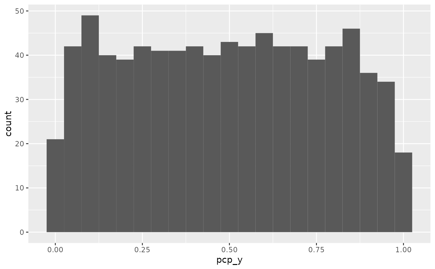
# y values are on five different values
table(pcp_data$pcp_y)
#> 
#>    0 0.25  0.5 0.75    1 
#>  232  210  301   61   22 

# spread out y values
pcp_data  |> pcp_arrange() |>
  ggplot(aes(x = pcp_y)) + geom_histogram(binwidth=0.05)