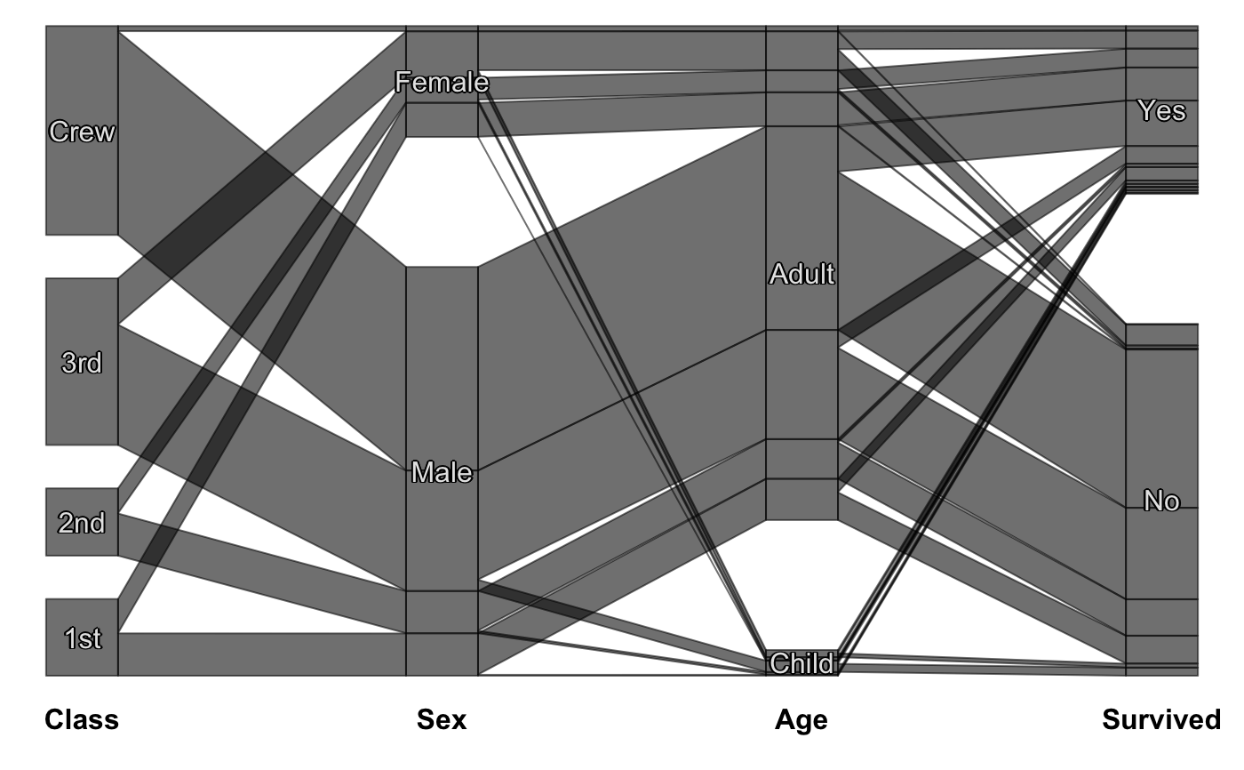
Static Categorical Parallel Coordinates Plot

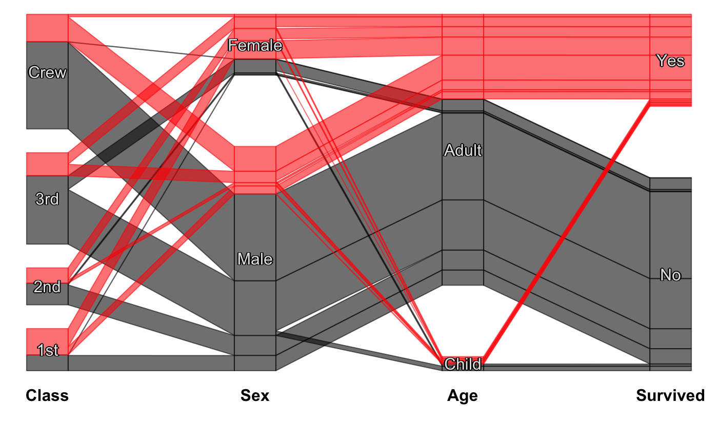
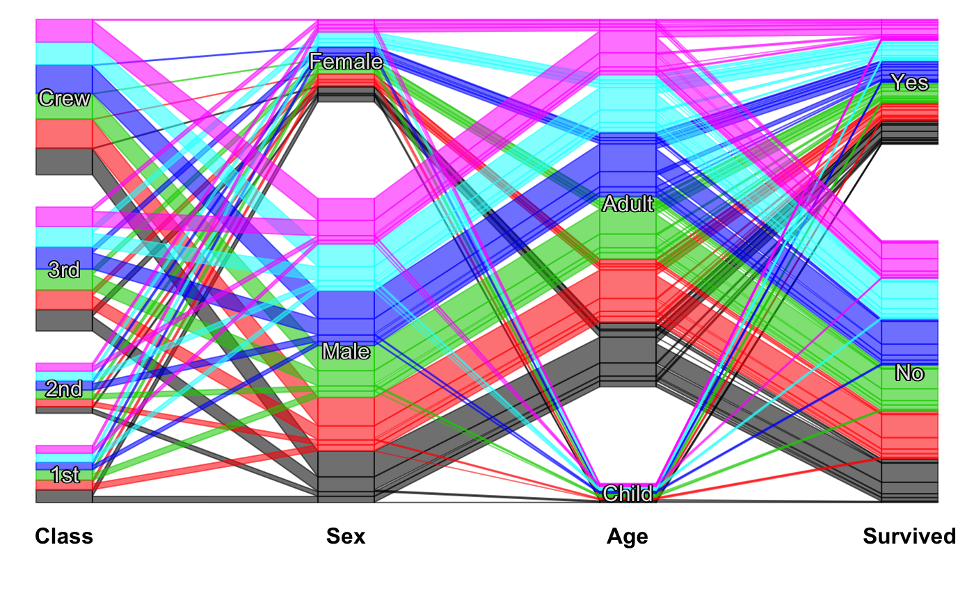
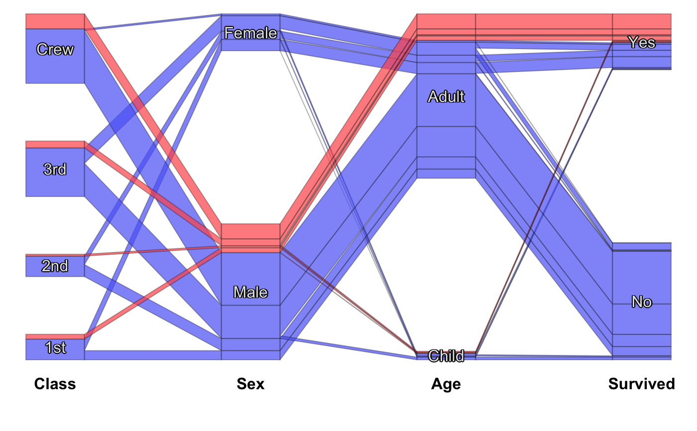
This function creates a static CPCP plot using base R graphics. The function offers color brush / highlighting and several options for the labels and colors. Efficiency is improved by replacing sets of parallel lines by polygons.

A ggplot version is under construction. A deprecated interactive version based on iplots (without labeling) is still available as extracat:::cpcp.

For reordering of category orders in CPCP plots see steptile.

scpcp(data, freqvar = "Freq", max.N = 1e6, gap = 0.2,
 sort.individual = TRUE, level.width = 0.2,
 polygon = TRUE, base.colour = alpha("black", 0.7), label = TRUE,
 lab.opt = list(rot = 0, col = 1, bg = TRUE, abbr = FALSE,
  abbr.var=12,hide.sel=TRUE, var.labels = TRUE),
 sel = NULL, sel.hide = TRUE, sel.palette = NULL,
 col.opt = list(), plot = TRUE, return.coords = !plot)

Arguments

data	The data.frame which can contain a variable called "Freq".
freqvar	Optional specification of a frequency variable.
max.N	The plot handles each case as a separate polyline, similar to conventional pcps. This option limits the number of observations.
gap	The size of the gaps between the categories as a total proportion.
sort.individual	Whether or not the cases (lines) are additionally rearranged according to the neighboring variable. This minimizes crossings.
level.width	The width of the rectangles representing the variables/categories.
polygon	Whether or not to replace parallel lines by polygons. This improves both efficiency and undesirable color effects.
base.colour	The standard color used for the cases which are not highlighted via sel.
label	Whether or not to draw category labels.
lab.opt	A list with options for the labels. See e.g. rmb
sel	A selection defining colors. This can either be an integer vector, a factor or an expression which returns such a vector. For instance sel="data[,4]" colors by the fourth variable, sel="sample(1:6,nrow(data),T)") leads to random colors and sel="Sex=='Male' & Survived=='Yes'" selects survivors among the men (in the titanic data, see examples). The objects (observations/lines) are additionally sorted by their color which brings colors together and makes it possible to see proportions of the selections.
sel.hide	Whether or not to hide the sel variable or plot it as the first variable.
sel.palette	The color palette for the selection. See getcolors.
col.opt	A list of options for the color palette. See getcolors.
plot	Whether or not to plot.
return.coords	Whether or not to return the coordinates per observation. plot = FALSE together with return.coords = FALSE is therefore rather stupid. The polygon coordinates are currently not returned.

Value

Either a logical value or the coordinates defining the polylines per observation.

References

Alexander Pilhoefer, Antony Unwin (2013). New Approaches in Visualization of Categorical Data: R Package extracat. Journal of Statistical Software, 53(7), 1-25. URL http://www.jstatsoft.org/v53/i07/

Note

A grid-based version is still under construction. In polygon mode single cases are still shown as a line rather than a ribbon of width 1/n.

See also

steptile

Examples

data(Titanic)
titanic <- as.data.frame(Titanic)

scpcp(titanic)

#scpcp(titanic, level.width=0)

#scpcp(titanic, gap=0)

#default with highlighting
scpcp(titanic, sel="data[,4]")

# random colors like for instance from a clustering
scpcp(titanic, sel="sample(1:6,nrow(data),T)")

# another one with some formal changes
require(scales)
scpcp(data=titanic,sel="Sex=='Male' & Survived=='Yes'", sel.palette = "w",
 col.opt=list(alpha=0.7,border=alpha(1,0.3)), gap = 0.5, level.width= 0.3)

# NOT RUN {
# mushroom data from the UCI machine learning repository
data(agaricus)
MR <- agaricus

levels(MR$stalk_root) <- c(levels(MR$stalk_root),"N/A")
MR$stalk_root[which(is.na(MR$stalk_root))] <- "N/A"

op <- optile(MR[,1:12], method="joint")


scpcp(op, sel = "odor",sel.palette="w",
         col.opt = list(border = alpha(1,0.1)), lab.opt=list(rot=45))


# ADAC ecotest data with four clusterings (k-means, mclust, hc Ward, hc complete)
data(eco)

# illustrate reordering success using coloring
scpcp(eco[,13:16], sel = "data[,1]", sel.palette="d")

scpcp(optile(eco[,13:16]), sel = "data[,1]", sel.palette="d",
         col.opt = list(border=alpha(1,0.1)))

# car classes (lower to upper class)
eco$Klasse <- factor(eco$Klasse, levels = levels(eco$Klasse)[c(3,1,2,7,4,5,6)])

scpcp(eco[,17:20], sel = eco$Klasse, sel.palette="s", col.opt = list(h=140))

# the color variable included
scpcp(eco[,c(3,17:20)], sel = eco$Klasse, sel.palette="s",
        col.opt = list(h=140),lab.opt = list(abbr=5))
# }