Hexagonal Binning and Piecharts

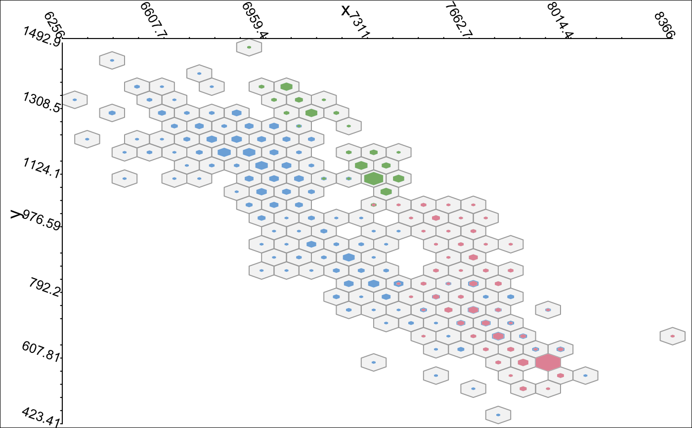
This function bins two continuous variables into a hexagonal grid and represents a third variable (which is usually a factor) via piecharts or nested hexagons within the bins. The main idea is to avoid overplotting and unfortunate effects that emerge from mixing up colors, e.g. with alpha-blending.

hexpie(x, y = NULL, z = NULL, n = 24, shape = "hex", p.rule = "radial",
decr.by.rank = NULL, freq.trans = I, alpha.freq = FALSE, col = "hcl",
col.opt = list(), show.hex = TRUE, random = NULL, xlim = range(x),
 ylim = range(y), label.opt = list(), vp = NULL)

Arguments

x	The variable for the horizontal axis. Should be integer or numeric.
y	The variable for the vertical axis. Should be integer or numeric.
z	The target variable for the colors which is handled as a factor.
n	The number of bins into which x is divided. See hexbin.
shape	There are two possibilities: "hex", "hexagonal", and "h" lead to hexagonal representations and "pie", "piechart", "circular" and "c" lead to circular representations.
p.rule	This controls the rules for the representation of the relative frequencies of the target categories. For shape = "hex" this should be one of "rad", "radius", "radial" meaning that the probabilities are represented by the radii. For shape = "circular" it is also possible to create piecharts via "angular", "angles" or "ang".
decr.by.rank	Whether or not to sort the categories within each hexagon individually by their frequencies in decreasing order. Defaults to NULL for no reordering but may be either TRUE (decreasing order) or FALSE (increasing order).
freq.trans	A function which is used to rescale the total counts of the cells. sqrt is a common choice.
alpha.freq	The frequencies may additionally be reflected in terms of the alpha values of the colors.
col	The choice of a color palette. See rmb for further explanations.
col.opt	Additional color options to replace the defaults. See rmb for further explanations.
show.hex	Whether or not to draw the hexagons. Setting col.opt = list(line.col.hex = NA) leaves the lines out and draws the background only.
random	If this is not NULL in each bin a random sample of n = random observations will be drawn (with replacement) from the corresponding data points. The resulting frequencies are then used to draw the piechart or hexagon. The main idea is to use random = 1 with larger numbers of bins such as n = 120 and show.hex = FALSE.
xlim	A vector of length 2 defining the x-limits e.g. computed via innerval .
ylim	A vector of length 2 defining the y-limits e.g. computed via innerval .
label.opt	Additional labeling options to replace the defaults. Not yet implemented.
vp	A viewport to plot in, e.g. for conditional plots.

Value

invisible(TRUE)

See also

stat_binhex, hexbin

Examples

data(olives)
x <- olives$oleic
y <- olives$linoleic
z <- olives$Region

# the default
hexpie(x,y,z)

# NOT RUN {
# zooming in (transformation of the total number of obs in each bin)
hexpie(x,y,z, freq.trans=sqrt)

# circular shapes
hexpie(x,y,z, freq.trans=sqrt, shape="pie")

# classical piecharts
hexpie(x,y,z, freq.trans=sqrt, shape="pie", p.rule ="angles")

#  the total numbers of obs are reflected via alpha-blending, 
# the grid is not shown and RGB colors are used
hexpie(x,y,z, freq.trans=sqrt, shape="hex", p.rule ="radial",
 alpha.freq=TRUE, col ="rgb",show.hex=F)

hexpie(x,y,z, freq.trans=NULL, shape="hex", p.rule ="radial",
 alpha.freq=TRUE, col ="rgb",show.hex=T)

require(ggplot2)
data(diamonds)
x2 <- diamonds$carat
y2 <- diamonds$price
z2 <- diamonds$color

# a standard plot with colors via ggplot2
qplot(x2,y2,colour=z2)

# the hexpie version
hexpie(x2,y2,z2,n=36)

# due to the few bins with the majority of observations
# it is sensible to zoom in
hexpie(x2,y2,z2,n=36,freq.trans=function(s) log(1+s))

# the same, but this time the central color is the most frequent one
hexpie(x2,y2,z2,n=36,freq.trans=function(s) log(1+s), decr.by.rank = TRUE)

# this way the difference is more obvious
# (although the color palette is better suited for ordinal target variables)

mat.layout <- grid.layout(nrow = 1 , ncol = 2 , widths = c(1/2,1/2), heights=1)
grid.newpage()
vp.mat <- viewport(layout = mat.layout)
pushViewport(vp.mat)

vp1 <- viewport(layout.pos.row = 1, layout.pos.col = 1)
pushViewport(vp1)

hexpie(x2,y2,z2,n=18,freq.trans=NULL,
        decr.by.rank=NULL,col="div", vp = vp1)

vp2 <- viewport(layout.pos.row = 1, layout.pos.col = 2)
pushViewport(vp2)

hexpie(x2,y2,z2,n=18,freq.trans=NULL,
        decr.by.rank=T,col="div", vp = vp1)
popViewport()

# random samples from the data (within bins) with many bins
# (takes some time)
require(scales)
grid.newpage()
hexpie(x2,y2,z2, freq.trans=function(s) log(1+s),random=1,
         n=240, show.hex=FALSE, col.opt=list(bg=alpha(1,0.7)),shape="c",col="rgb")
# }