facetshade

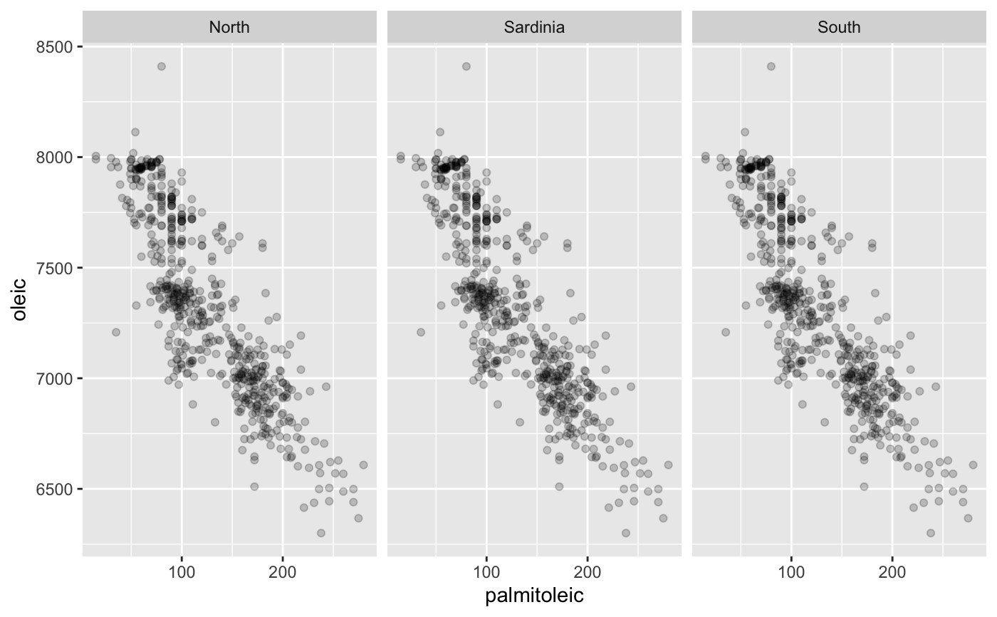
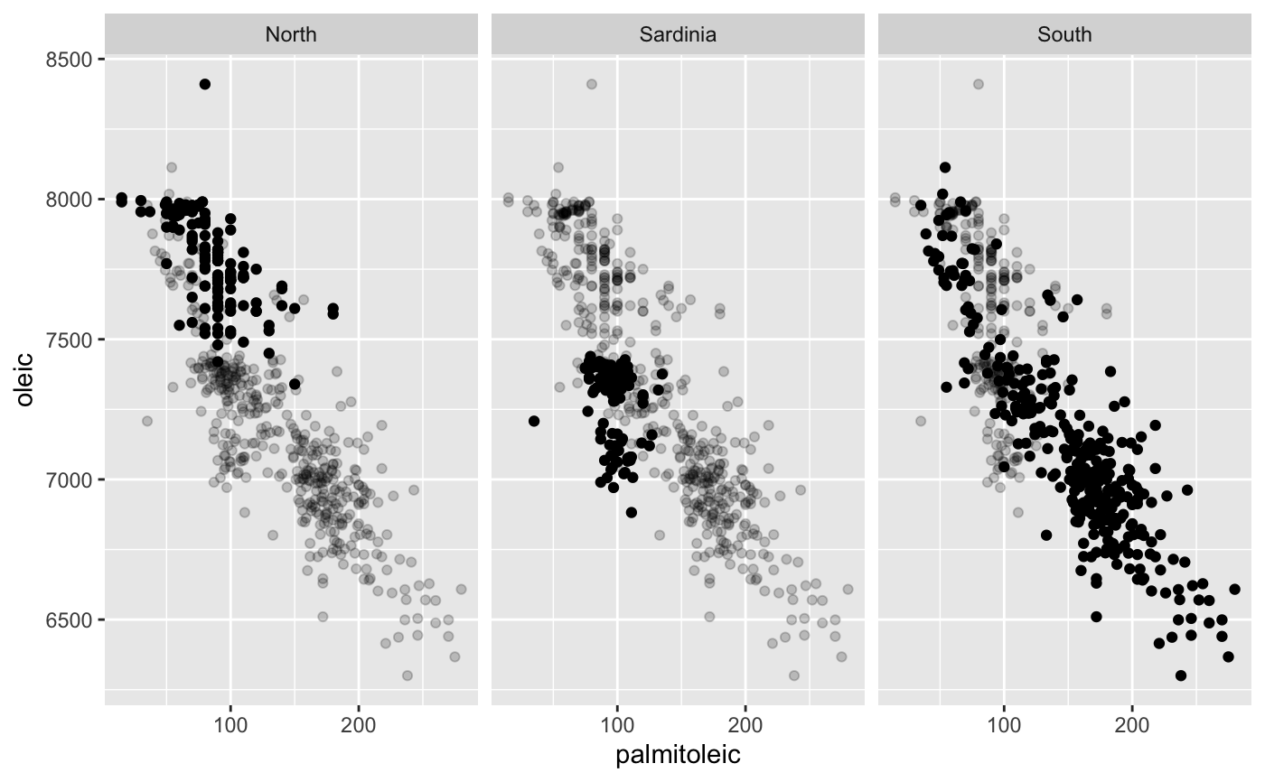
This function makes it possible to create ggplots using facet_grid with a plot of the complete data in the background of each facet. There are two options: If geom is specified then the background data is put into a separate layer. The original data is stored in the main object. The other option is to not specify a geom. In this case the modified data is stored in the main body. See examples.

facetshade( data, mapping, f, geom, geom.mapping, bg.all = TRUE, keep.orig = FALSE, ...)

Arguments

data	The dataframe used for the background plots in the first layer.
mapping	The aesthetic mapping conctructed via aes.
f	The formula specifying the grid for facet_grid or a facet/wrap.
geom	The geom used for the shade.
geom.mapping	Aesthetics for the shade.
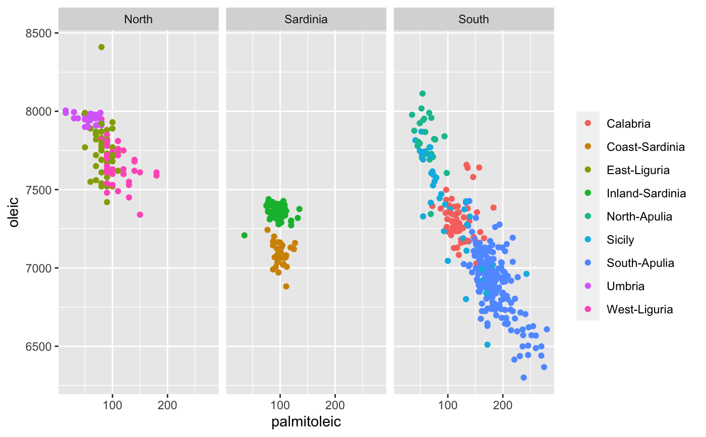
bg.all	Whether or not to use all data points for each background plot. If `FALSE` then the data for the background is the compleent of the data in the facet.
keep.orig	Logical. Whether to keep the original faceting variables defined by `f`. Those are renamed by adding `orig.` as a prefix. For example `f = .~variable` will work fine with `group = orig.variable`. See FinCal example.
…	Further arguments for the background layer or the main ggplot object.

Value

A ggplot object.

Examples


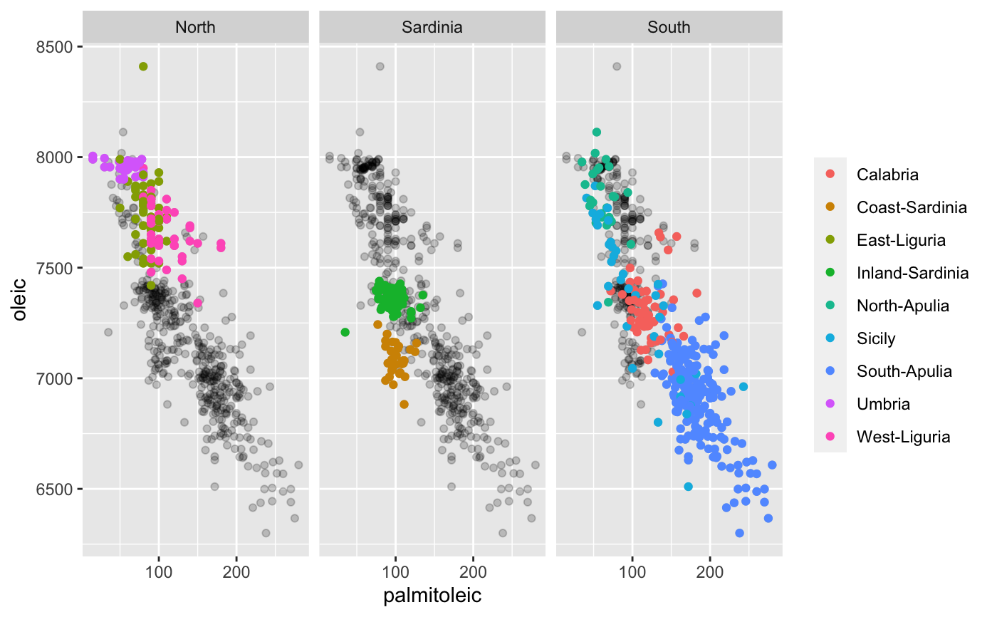
# produces a modified data.frame mdata and returns:
# ggplot(data = mdata, mapping, ... ) + facet_grid(f)

require(scales)
require(ggplot2)
#> Loading required package: ggplot2

# facetshade object:
fs1 <- facetshade( data = olives, aes(x = palmitoleic, y = oleic),
        f = .~Region )

# only the background-data
fs1 + geom_point( colour = alpha(1, 0.2) )

# the actual data added in a second layer:
fs1 + geom_point( colour = alpha(1, 0.2) ) +
geom_point( data = olives )

# now again with colours:
fs1 + geom_point( colour = alpha(1, 0.2) ) +
geom_point( data = olives, aes(colour = Area) )

# a different geom for the background-plot:
fs1 + geom_density2d(colour=alpha(1,0.1)) +
geom_point( data = olives, aes(colour = Area) )
#> Warning: Computation failed in `stat_density2d()`:
#> there is no package called ‘isoband’
#> Warning: Computation failed in `stat_density2d()`:
#> there is no package called ‘isoband’
#> Warning: Computation failed in `stat_density2d()`:
#> there is no package called ‘isoband’
# NOT RUN {
# OPTION 2: specify geom in facetshade call:
fs1b <- facetshade( data = olives, aes(x = palmitoleic, y = oleic),
        f = .~Region , geom = geom_point)
fs1b + geom_point(aes(colour = Area))
# }

# compare with complement:
fs2 <- facetshade( data = olives, aes(x = palmitoleic, y = oleic),
         f = .~Region , bg.all = FALSE)

fs2 + geom_density2d(colour=alpha(1,0.1)) +
geom_point( data = olives, aes(colour = Area) )
#> Warning: Computation failed in `stat_density2d()`:
#> there is no package called ‘isoband’
#> Warning: Computation failed in `stat_density2d()`:
#> there is no package called ‘isoband’
#> Warning: Computation failed in `stat_density2d()`:
#> there is no package called ‘isoband’
# NOT RUN {
# OPTION 2: specify geom in facetshade call:
fs2b <- facetshade( data = olives, aes(x = palmitoleic, y = oleic),
        f = .~Region , geom = geom_density2d, bg.all = FALSE)
fs2b + geom_point(aes(colour = Area))
# }

# a second dataset:
# NOT RUN {
data(EURO4PlayerSkillsSep11, package="SportsAnalytics")
e4 <- subset(EURO4PlayerSkillsSep11,Attack > 0 & Defence > 0)


fs3 <- facetshade( data = e4, aes(x = Attack, y = Defence),
        f = .~Position , compare.all = TRUE)

fs3 + geom_point( colour = alpha(1, 0.1) ) +
geom_point( data = e4, aes(colour = Position) ,alpha=0.3)

fs3 + geom_bin2d( colour = alpha(1, 0.1) ) +
geom_point( data = e4, aes(colour = Position) ,alpha=0.3)

# now with two facet variables
fs4 <- facetshade( data = e4, aes(x = Attack, y = Defence),
        f = Position~Side , compare.all = TRUE)

fs4 + geom_point( colour = alpha(1, 0.1) ) +
geom_point( data = e4, aes(colour = Position))
# }
# NOT RUN {
library(FinCal)
sh13 <- get.ohlcs.google(symbols=c("AAPL","GOOG","IBM", "MSFT"),
start="2013-01-01",end="2013-12-31")

# OPTION 1 ------------
require(reshape2)
SH13 <- data.frame(date = as.Date(sh13$AAPL$date),
 sapply(sh13,"[" ,"close",USE.NAMES=TRUE))

names(SH13) <- c("date",names(sh13))
SH13[,-1] <- apply(SH13[,-1], 2, function(x) 100*x/x[1])
SH13am <- melt(SH13, id="date")


# OPTION 2 ------------ 
#SH13am <- do.call(rbind,
#		 mapply(function(z,y){
#		 		data.frame(
#		 			date = as.Date(z$date),
#		 			value = 100*z$close/z$close[1],
#		 			variable = y)
#		 } , z = sh13, y = names(sh13), SIMPLIFY = FALSE))
# ---------------------		


# original plot from GDAR:
ggplot(SH13am, aes(date, y=value, colour=variable,group=variable)) +
geom_line()+ xlab("") + ylab("") +
 theme(legend.position="bottom") +
 theme(legend.title=element_blank())


# facetshade:
# compare to "average" of others:
facetshade(SH13am,aes(x=date, y=value),f = .~variable, bg.all = FALSE) +
 geom_smooth(aes(x=date, y=value),method="loess",span = 1/28) +
 geom_line(data=SH13am,aes(colour=variable),show_guide=FALSE) +
 xlab("") + ylab("")

# compare to all others
facetshade(SH13am,aes(x=date, y=value),
 f = .~variable, bg.all = FALSE,keep.orig = TRUE) +
 geom_line(aes(x=date, y=value,group=orig.variable),colour = alpha(1,0.3)) +
 geom_line(data=SH13am,aes(colour=variable),show_guide=FALSE, size = 1.2) +
xlab("") + ylab("")

# --- parallel coordinates --- #

sc <- scale(olives[,3:10])

# OPT: order by var
ord <- order(apply(sc,2,sd))
sc <- sc[,ord]

require(scales)
# OPT: align at median
sc <- apply(sc,2,function(z) rescale_mid(z, mid = median(z,na.rm=TRUE)))



require(reshape2)
require(ggplot2)

msc <- melt(sc)
msc$Area <- olives$Area


f1 <- facetshade(msc,aes(x=Var2,y=value,group=Var1),f=.~Area, bg.all = FALSE)
f1+geom_line(alpha=0.05)+
geom_line(data=msc,aes(colour=Area),alpha=0.2)+
facet_wrap(f=~Area,nrow=3)

# }# NOT RUN {
        # TESTCODE: instead of creating a new object
        # a shade layer is added to an existing ggplot
        # NOTE: function CHANGES the object!

# highlighting + alpha
pp0 <- ggplot()+geom_point(data = olives,
 aes(x = palmitoleic, y = palmitic), colour = 2) + facet_wrap(~Area, ncol = 3)
        extracat:::facetshade2(pp0, alpha = 0.1, colour = 1)

# colours for both, alpha for shade	
pp1 <- ggplot()+geom_point(data = olives,
 aes(x = palmitoleic, y = oleic, colour = Area)) + facet_grid(.~Region)
        extracat:::facetshade2(pp1, alpha = 0.1)

# different geom and colour for shade	
pp2 <- ggplot()+geom_point(data = olives,
 aes(x = palmitoleic, y = oleic, colour = Area)) + facet_grid(.~Region)
        extracat:::facetshade2(pp2, geom = geom_density2d,
         mapping = aes(colour = NULL), colour = 7)

# smooth over points shade with matching colours
pp3 <- ggplot()+geom_smooth(data = olives,
 aes(x = palmitoleic, y = oleic, colour = Region)) + facet_grid(.~Region)
        extracat:::facetshade2(pp3, geom = geom_point,
         mapping = aes(colour = orig.Region), keep.orig = TRUE)

# }

Arguments

Value

See also

Examples

Contents

Author