Reading Files

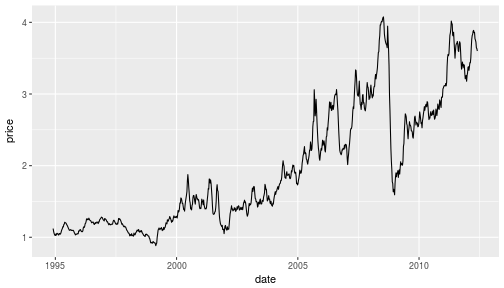
class: center, middle, inverse, title-slide

# Reading Files
### Haley Jeppson, Sam Tyner

---

## Data in Excel

- Formats xls and csv - what's the difference?

- File extensions xls and xlsx are proprietary Excel formats, binary files

- csv is an extension for Comma Separated Value files. They are text files - directly readable.

- Example: Gas prices in midwest since 1994

---

## Gas Prices in the Midwest

```r
library(readr)
midwest <- read_csv("http://heike.github.io/rwrks/03-r-format/data/midwest.csv")
head(midwest)
```

```
## # A tibble: 6 x 11
##   `Year-Month` `Week 1` X3    `Week 2` X5    `Week 3` X7    `Week 4` X9   
##   <chr>        <chr>    <chr> <chr>    <chr> <chr>    <chr> <chr>    <chr>
## 1 <NA>         End Date Value End Date Value End Date Value End Date Value
## 2 1994-Nov     <NA>     <NA>  <NA>     <NA>  <NA>     <NA>  28-Nov   1.122
## 3 1994-Dec     5-Dec    1.086 12-Dec   1.057 19-Dec   1.039 26-Dec   1.027
## 4 1995-Jan     2-Jan    1.025 9-Jan    1.046 16-Jan   1.031 23-Jan   1.054
## 5 1995-Feb     6-Feb    1.045 13-Feb   1.04  20-Feb   1.031 27-Feb   1.052
## 6 1995-Mar     6-Mar    1.053 13-Mar   1.042 20-Mar   1.048 27-Mar   1.065
## # ... with 2 more variables: `Week 5` <chr>, X11 <chr>
```

---
## `read_csv` vs. `read_*`

`read_csv` is just one way to read a file using the `readr` package:

- `read_delim`: the most generic function. Use the `delim` argument to read a file with any type of delimiter 
- `read_tsv`: read tab separated files 
- `read_lines`: read a file into a vector that has one element per line of the file
- `read_file`: read a file into a single character element
- `read_table`: read a file separated by space

---
class: inverse
## Your Turn

Have a look at the parameters of `read_csv` to solve the following problems:

1. Read the first two lines of the file into an object called `midwest_names`

2. Read everything EXCEPT the first two lines into an object called `midwest_data`

Hint: Visit http://heike.github.io/rwrks/03-r-format/data/midwest.csv to download the data and look at it in Excel to help figure out what the issue is.

---

## Quick Lesson in Data Cleaning

```r
library(lubridate)
library(tidyverse)
values <- c(midwest_data$X3, midwest_data$X5, midwest_data$X7, 
            midwest_data$X9, midwest_data$X11)
dates <- c(paste(midwest_data$X1, midwest_data$X2, sep = "-"), 
           paste(midwest_data$X1, midwest_data$X4, sep = "-"),
           paste(midwest_data$X1, midwest_data$X6, sep = "-"),
           paste(midwest_data$X1, midwest_data$X8, sep = "-"),
           paste(midwest_data$X1, midwest_data$X10, sep = "-"))

dates <- dates[!is.na(values)]
values <- values[!is.na(values)]

dates <- ymd(dates)

midwest_gas <- data_frame(date = dates, price = values)
midwest_gas <- arrange(midwest_gas, dates)
```

---

## Now we can make a plot!

```r
library(ggplot2)
ggplot(midwest_gas, aes(x = date, y = price)) + geom_line()
```

![](1-Files_files/figure-html/unnamed-chunk-4-1.png)

---

## Reading Excel Data

Download the midwest.xls file to your current working directory (`getwd()`)

```r
library(readxl)

midwest2 <- read_excel("midwest.xls")

head(midwest2)
```

Something isn't quite right here...

```
## # A tibble: 6 x 11
##   `Year-Month` `Week 1` X__1  `Week 2` X__2  `Week 3` X__3  `Week 4` X__4 
##   <chr>        <chr>    <chr> <chr>    <chr> <chr>    <chr> <chr>    <chr>
## 1 <NA>         End Date Value End Date Value End Date Value End Date Value
## 2 1994-Nov     <NA>     <NA>  <NA>     <NA>  <NA>     <NA>  39779    1.122
## 3 1994-Dec     39786    1.086 39793    1.057 39800    1.039 39807    1.027
## 4 1995-Jan     39448    1.025 39455    1.046 39462    1.031 39469    1.054
## 5 1995-Feb     39483    1.045 39490    1.04  39497    1.031 39504    1.052
## 6 1995-Mar     39512    1.053 39519    1.042 39526    1.048 39533    1.065
## # ... with 2 more variables: `Week 5` <chr>, X__5 <chr>
```

---

## Reading Excel Data: Attempt #2

The 2nd row of the excel file also contains variable names.

Let's skip the first this time. We can then rename the first column.

```r
library(readxl)

midwest2 <- read_excel("midwest.xls", skip = 1)
names(midwest2)[1] <- "Year-Month"
head(midwest2)
```

```
## # A tibble: 6 x 11
##   `Year-Month` `End Date`          Value `End Date__1`       Value__1
##   <chr>        <dttm>              <dbl> <dttm>                 <dbl>
## 1 1994-Nov     NA                  NA    NA                     NA   
## 2 1994-Dec     2012-12-05 00:00:00  1.09 2012-12-12 00:00:00     1.06
## 3 1995-Jan     2012-01-02 00:00:00  1.02 2012-01-09 00:00:00     1.05
## 4 1995-Feb     2012-02-06 00:00:00  1.04 2012-02-13 00:00:00     1.04
## 5 1995-Mar     2012-03-06 00:00:00  1.05 2012-03-13 00:00:00     1.04
## 6 1995-Apr     2012-04-03 00:00:00  1.09 2012-04-10 00:00:00     1.11
## # ... with 6 more variables: `End Date__2` <dttm>, Value__2 <dbl>, `End
## #   Date__3` <dttm>, Value__3 <dbl>, `End Date__4` <dttm>, Value__4 <dbl>
```

Better, but not yet perfect...

---

## `foreign` Package

- Other file formats can be read using the functions from package `foreign`

- SPSS: `read.spss`

- SAS: `read.xport`

- Minitab: `read.mtp`

- Systat: `read.systat`

---
class: inverse
## Your Turn (~2 minutes)

The NHANES (National Health and Nutrition Survey) publishes data in the SAS xport format:

https://wwwn.cdc.gov/Nchs/Nhanes/continuousnhanes/default.aspx?BeginYear=2013

1. Scroll to the bottom, choose one of the datasets (Demographics, Examination, etc.). Download the Data file (XPT)

2. Use `read.xport()` to load the file into R

3. Briefly examine the dataset you've imported (use `head` or `tail`, etc)