Data Visualization

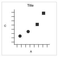
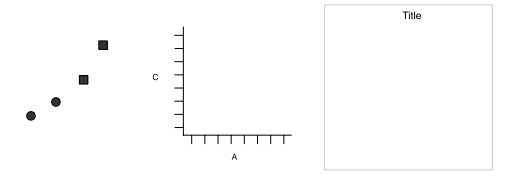
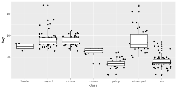
class: center, middle, inverse, title-slide

# Data Visualization
## Using ggplot2
### Haley Jeppson and Sam Tyner

---

class: center, middle

# BUILDING PLOTS

---
class: inverse, center, middle

# Underlying theory

---

# What is a graphic?

ggplot2 uses the idea that you can build every graph from the same components:

1. a **data** set
  
  2. a **coordinate system**
  
  3. **geoms** - visual marks that represent data
  
- to display values, map variables in the data to visual properties of the geom (**aesthetics**) like **size**, **color**, and **x** and **y** locations

![](images/build1.png)![](images/build2.png)

---
# How to build a graph

Complete the template below to build a graph
<img src="3-Layers_files/figure-html/unnamed-chunk-2-1.png"  />

---
# How to build a graph

`ggplot(data = mpg, aes(x = cty, y = hwy))`

- This will begin a plot that you can finish by adding layers to.

- You can add one geom per layer

---
class: inverse
## Your Turn

Change the code below to have the points **on top** of the boxplots.

```r
ggplot(data = mpg, aes(x = class, y = hwy)) + 
  geom_jitter() + 
  geom_boxplot()
```

![](3-Layers_files/figure-html/unnamed-chunk-4-1.png)
---

# What is a geom?

In ggplot2, we use a geom function to represent data points, and use the geom's aesthetic properties to represent variables.

Once our data is formatted and we know what type of variables we are working with, we can select the correct geom for our visualization.

---
## Available geoms

---
# What is a layer?

- it determines the physical representation of the data

- Together, the data, mappings, statistical transformation, and geometric object form a layer

- A plot may have multiple layers
 
<img src="3-Layers_files/figure-html/unnamed-chunk-8-1.png"  />

---
# Alternative method of building layers: Stats

A stat builds a new variable to plot (e.g., count and proportion)
.pull-left[
<img src="3-Layers_files/figure-html/unnamed-chunk-10-1.png"  />
]
.pull-right[
<img src="3-Layers_files/figure-html/unnamed-chunk-11-1.png"  />
]

---

# Faceting

A way to extract subsets of data and place them side-by-side in graphics

```r
ggplot(data = mpg, aes(x = cty, y = hwy, colour = class)) + geom_point()

ggplot(data = mpg, aes(x = cty, y = hwy, colour = class)) + geom_point() +facet_grid(.~class)
```

---
# Faceting Options

- `facet_grid(. ~ b)`:facet into columns based on b 
- `facet_grid(a ~ .)`:facet into columns based on a 
- `facet_grid(a ~ b)`:facet into both rows and columns
- `facet_wrap( ~ fl)`:wrap facets into a rectangular layout

You can set scales to let axis limits vary across facets:

- `facet_grid(y ~ x, scales = "free")`: x and y axis limits adjust to individual facets
- "free_x" - x axis limits adjust
- "free_y" - y axis limits adjust

You can also set a labeller to adjust facet labels:
- `facet_grid(. ~ fl, labeller = label_both)`
- `facet_grid(. ~ fl, labeller = label_bquote(alpha ^ .(x)))`
- `facet_grid(. ~ fl, labeller = label_parsed)`

---

# Position Adjustments

Position adjustments determine how to arrange geoms that would otherwise occupy the same space
- **Dodge**: Arrange elements side by side 
- **Fill**: Stack elements on top of one another, normalize height
- **Stack**: Stack elements on top of one another

`ggplot(mpg, aes(fl, fill = drv)) + geom_bar(position = "")`

---
# Position Adjustments: Jitter

- **Jitter**: Add random noise to X & Y position of each element to avoid overplotting
- There is also a jitter geom

---

## Coordinate Systems

- `coord_cartesian()`: The default cartesian coordinate system
- `coord_fixed()`: Cartesian with fixed aspect ratio between x & y units
- `coord_flip()`: Flipped Cartesian coordinates
- `coord_polar()`: Polar coordinates
- `coord_trans()`: Transformed cartesian coordinates.
- `coord_map()`: Map projections from the mapproj package (mercator (default), azequalarea, lagrange, etc.)

---

## ggplot2 extenstions

[gallery](https://exts.ggplot2.tidyverse.org/)