class: center, middle, inverse, title-slide # Motivating Example ### Haley Jeppson and Sam Tyner --- ## Motivating Example - Kick off the workshop by exploring a real data set using R! -- - Goal: get the flavor of using R for data management and exploration -- - Don't worry about understanding all the coding right away - We will go back and explain how it all works in detail - Follow along using [2-MotivatingExample.R](../code/2-MotivatingExample.R) --- ## Getting Started Let's begin by installing and loading `tidyverse`: ```r install.packages("tidyverse") library(tidyverse) ``` This workshop will focus largely on a group of packages that live together under the name `tidyverse`. `tidyverse` includes the following well known packages: - `ggplot2` - `dplyr` - `tidyr` - `readr` - and more! --- ## Salmonella Shedding Data - Fecal *Salmonella* shedding recorded over the course of 21 days - Several **variables** were recorded for each pig at certain time points: - Amount of *Salmonella* in feces (log10) - Pig weight (kg) - Dietary treatment group - **Primary Question**: Do the different dietary treatments affect *Salmonella* shedding? --- ## First look at data in R Lets use R to look at the top few rows of the *Salmonella* shedding data set. First, we load tip using `read_csv`: ```r shed <- read_csv("http://heike.github.io/rwrks/01-r-intro/data/daily_shedding.csv") ``` Now, we use the `head` function to look at the first 6 rows of the data: ```r head(shed) ``` ``` ## # A tibble: 6 x 12 ## pignum time_point pig_weight temp pan_wt wet_wt Dry_wt_pan Dry_weight ## <int> <int> <dbl> <dbl> <dbl> <dbl> <dbl> <dbl> ## 1 77 2 NA 103 1.02 1.09 1.31 0.290 ## 2 87 2 NA 104 1.04 1.02 1.33 0.290 ## 3 122 2 NA 104 1.02 0.990 1.11 0.0900 ## 4 160 2 NA 104 1.09 1.00 1.36 0.270 ## 5 191 2 NA 104 1.03 1.02 1.27 0.240 ## 6 224 2 NA 103 1.08 1.00 1.39 0.310 ## # ... with 4 more variables: percent_drymatter <dbl>, ## # daily_shedding <dbl>, treatment <chr>, total_shedding <dbl> ``` --- ## *Salmonella* Shedding Data: Attributes How big is this data set and what types of variables are in each column? ```r str(shed) ``` ``` ## Classes 'tbl_df', 'tbl' and 'data.frame': 295 obs. of 12 variables: ## $ pignum : int 77 87 122 160 191 224 337 345 419 458 ... ## $ time_point : int 2 2 2 2 2 2 2 2 2 2 ... ## $ pig_weight : num NA NA NA NA NA NA NA NA NA NA ... ## $ temp : num 103 104 104 104 104 ... ## $ pan_wt : num 1.02 1.04 1.02 1.09 1.03 1.08 1.03 1.09 1.07 1.04 ... ## $ wet_wt : num 1.09 1.02 0.99 1 1.02 1 1.02 0.99 1.07 1.06 ... ## $ Dry_wt_pan : num 1.31 1.33 1.11 1.36 1.27 1.39 1.3 1.24 1.38 1.26 ... ## $ Dry_weight : num 0.29 0.29 0.09 0.27 0.24 0.31 0.27 0.15 0.31 0.22 ... ## $ percent_drymatter: num 26.61 28.43 9.09 27 23.53 ... ## $ daily_shedding : num 5.3 5.7 13.22 6.75 5.86 ... ## $ treatment : chr "control" "control" "control" "control" ... ## $ total_shedding : num 2.3 2.48 5.74 2.93 2.54 ... ## - attr(*, "spec")=List of 2 ## ..$ cols :List of 12 ## .. ..$ pignum : list() ## .. .. ..- attr(*, "class")= chr "collector_integer" "collector" ## .. ..$ time_point : list() ## .. .. ..- attr(*, "class")= chr "collector_integer" "collector" ## .. ..$ pig_weight : list() ## .. .. ..- attr(*, "class")= chr "collector_double" "collector" ## .. ..$ temp : list() ## .. .. ..- attr(*, "class")= chr "collector_double" "collector" ## .. ..$ pan_wt : list() ## .. .. ..- attr(*, "class")= chr "collector_double" "collector" ## .. ..$ wet_wt : list() ## .. .. ..- attr(*, "class")= chr "collector_double" "collector" ## .. ..$ Dry_wt_pan : list() ## .. .. ..- attr(*, "class")= chr "collector_double" "collector" ## .. ..$ Dry_weight : list() ## .. .. ..- attr(*, "class")= chr "collector_double" "collector" ## .. ..$ percent_drymatter: list() ## .. .. ..- attr(*, "class")= chr "collector_double" "collector" ## .. ..$ daily_shedding : list() ## .. .. ..- attr(*, "class")= chr "collector_double" "collector" ## .. ..$ treatment : list() ## .. .. ..- attr(*, "class")= chr "collector_character" "collector" ## .. ..$ total_shedding : list() ## .. .. ..- attr(*, "class")= chr "collector_double" "collector" ## ..$ default: list() ## .. ..- attr(*, "class")= chr "collector_guess" "collector" ## ..- attr(*, "class")= chr "col_spec" ``` --- ## *Salmonella* Shedding: Variables Let's get a summary of the values for each variable: ```r summary(shed) ``` ``` ## pignum time_point pig_weight temp ## Min. : 6.0 Min. : 0.0 Min. : 9.48 Min. :101.2 ## 1st Qu.:119.0 1st Qu.: 2.0 1st Qu.:16.02 1st Qu.:102.4 ## Median :224.0 Median : 7.0 Median :19.78 Median :102.9 ## Mean :234.7 Mean : 8.8 Mean :21.01 Mean :102.9 ## 3rd Qu.:361.0 3rd Qu.:14.0 3rd Qu.:25.29 3rd Qu.:103.4 ## Max. :472.0 Max. :21.0 Max. :36.30 Max. :105.2 ## NA's :59 NA's :118 ## pan_wt wet_wt Dry_wt_pan Dry_weight ## Min. :1.000 Min. :0.700 Min. :1.110 Min. :0.090 ## 1st Qu.:1.030 1st Qu.:1.000 1st Qu.:1.300 1st Qu.:0.250 ## Median :1.050 Median :1.020 Median :1.320 Median :0.280 ## Mean :1.054 Mean :1.026 Mean :1.322 Mean :0.268 ## 3rd Qu.:1.070 3rd Qu.:1.050 3rd Qu.:1.353 3rd Qu.:0.290 ## Max. :1.120 Max. :1.110 Max. :1.460 Max. :0.380 ## NA's :122 NA's :123 NA's :123 NA's :123 ## percent_drymatter daily_shedding treatment total_shedding ## Min. : 9.091 Min. : 0.000 Length:295 Min. : 0.000 ## 1st Qu.:24.292 1st Qu.: 0.000 Class :character 1st Qu.: 1.699 ## Median :26.923 Median : 3.912 Mode :character Median :13.904 ## Mean :26.109 Mean : 3.765 Mean :17.423 ## 3rd Qu.:28.431 3rd Qu.: 5.521 3rd Qu.:30.893 ## Max. :36.893 Max. :13.218 Max. :66.207 ## NA's :123 ``` --- ## Scatterplots Lets look at the relationship between time point and *Salmonella* shedding. ```r ggplot(shed, aes(x=time_point, y=total_shedding)) + geom_point() ``` 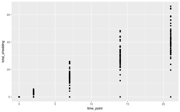<!-- --> --- ## More Scatterplots Color the points by treatment groups ```r ggplot(shed, aes(x=time_point, y=total_shedding, colour = treatment)) + geom_point() ``` 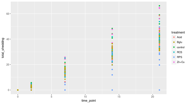<!-- --> --- ## More Scatterplots Switch to lines for easier reading ```r ggplot(shed, aes(x=time_point, y=total_shedding, colour = treatment)) + geom_line(aes(group=pignum)) ``` 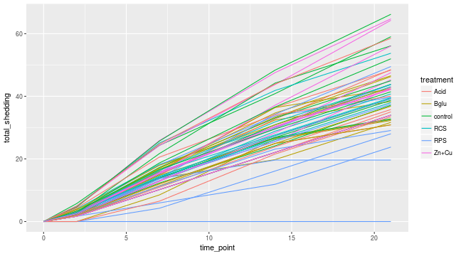<!-- --> --- ## Even More Plots Add facetting ```r ggplot(shed, aes(x=time_point, y=total_shedding, color=treatment)) + geom_line(aes(group=pignum)) + facet_wrap(~treatment) ``` 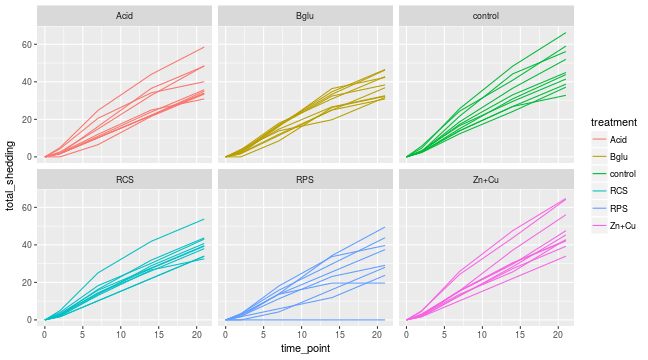<!-- --> --- ## Variable Creation and Data Filtering We will make a new variable in the data: `gain = weight at day 21 - weight at day 0`. We will then filter the data to only include the final values. ```r final_shed <- shed %>% group_by(pignum) %>% mutate(gain = pig_weight[time_point == 21] - pig_weight[time_point == 0]) %>% filter(time_point == 21) %>% ungroup() %>% select(-c(4:9)) summary(final_shed$gain) ``` ``` ## Min. 1st Qu. Median Mean 3rd Qu. Max. ## 8.22 12.40 14.14 14.16 16.04 18.86 ``` --- ## Histogram Lets look distribution of the final shedding values with a histogram ```r ggplot(final_shed) + geom_histogram(aes(x = total_shedding)) ``` ``` ## `stat_bin()` using `bins = 30`. Pick better value with `binwidth`. ``` <!-- --> --- ## One pig did not shed at all... which pig and what treatment did it receive? ```r final_shed[which.min(final_shed$total_shedding),] ``` ``` ## # A tibble: 1 x 7 ## pignum time_point pig_weight daily_shedding treatment total_shedding ## <int> <int> <dbl> <dbl> <chr> <dbl> ## 1 97 21 24.9 0 RPS 0 ## # ... with 1 more variable: gain <dbl> ``` --- ## Shedding by Treatment Look at the average cumulative shedding value for each treatment seperately ```r # Using base `R`: median(final_shed$total_shedding[final_shed$treatment == "control"]) ``` ``` ## [1] 44.42518 ``` ```r # then repeat for each treatment. Or ... ``` ```r # Using `tidyverse`: final_shed %>% group_by(treatment) %>% summarise(med_shed = median(total_shedding)) ``` ``` ## # A tibble: 6 x 2 ## treatment med_shed ## <chr> <dbl> ## 1 Acid 35.4 ## 2 Bglu 37.6 ## 3 control 44.4 ## 4 RCS 39.4 ## 5 RPS 29.1 ## 6 Zn+Cu 44.1 ``` ] --- ## Statistical Significance There is a difference but is it statistically significant? ```r wilcox.test(total_shedding ~ treatment, data = final_shed, subset = treatment %in% c("control", "RPS")) ``` ``` ## ## Wilcoxon rank sum test ## ## data: total_shedding by treatment ## W = 75, p-value = 0.01327 ## alternative hypothesis: true location shift is not equal to 0 ``` --- ## Boxplots We could compare the cumulative shedding values of each treatment group with a side by side boxplot ```r ggplot(final_shed) + geom_boxplot( aes(treatment, total_shedding, fill = treatment)) ``` <!-- --> --- ## Boxplots Again Alternatively, we could use the original data to compare the daily shedding values of each treatment group with a side by side boxplot over time ```r shed %>% filter(time_point != 0) %>% ggplot() + geom_boxplot( aes(treatment, daily_shedding, fill = treatment), position = "dodge") + facet_wrap(~time_point) ``` <!-- --> --- class: inverse ## Your Turn Try playing with chunks of code from this session to further investigate the *Salmonella* shedding data: 1. Get a summary of the daily shedding values (use the `shed` data set) 2. Make side by side boxplots of final weight gain by treatment group (use the `final_shed` data set) 3. Compute a wilcox test for control vs. the "Bglu" treatment group